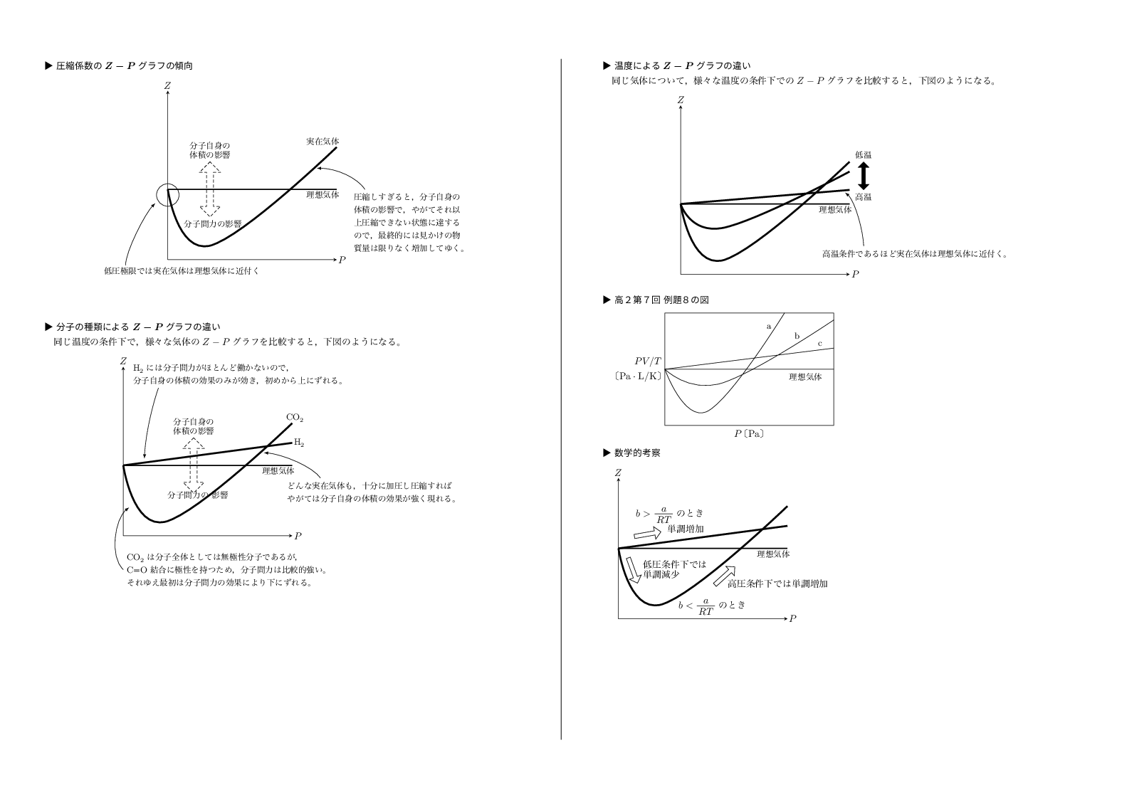
圧縮係数の$Z-P$グラフの傾向

\documentclass[b4j,9pt,twocolumn,landscape]{tetsujsarticle}
\usepackage{tetsuchem}
\pagestyle{fancy}

\余白設定[
上余白=1truecm,
下余白=上余白,
左余白=1.414truecm,
左右差=0truecm,
段間隔=対称,
段組の仕切り線の太さ=.5truept,
ヘッダの縦幅=16truept,
ヘッダ下端と本文上端の縦間隔=10truept,
ヘッダと本文を仕切る線の太さ=0truept,
本文下端とフッタ下端の縦間隔=20truept,
本文とフッタを仕切る線の太さ=0truept,
傍注領域の幅=0truept,
本文端と傍注領域との間隔=0truept,
傍注同士の縦間隔=\baselineskip,
奇数ページの傍注位置=右,
偶数ページの傍注位置=左,
]


\begin{document}

\小見出し{圧縮係数の$Z-P$グラフの傾向}

\begin{center}
\begin{tikzpicture}[>=stealth]
\draw[->] (0,0) -- (6,0) node at +(0.2,0) {$P$};
\draw[->] (0,0) -- (0,6) node at +(0,0.2) {$Z$};
\draw[line width=1pt] (0,2.5) -- (6,2.5) node at +(-0.5,-0.2) {\small 理想気体};
\draw (0,2.3) circle (0.4cm) ;
\node at (5.5,4.2) {\small 実在気体};
\node[double arrow,draw,densely dashed,rotate=90] (arrow) at (1.5,2.5) {\hbox{\ihspace{4.5zw}}};
\node at ($(arrow)+(0.1,-1.22)$) {\small 分子間力の影響};
\node at ($(arrow)+(0,1.4)$) {\small\parbox{5zw}{\baselineskip=0pt 分子自身の\\体積の影響}};
\pgfsetlinewidth{1.75pt}
\pgfsetplottension{0.7}
\pgfplothandlercurveto
\pgfplotstreamstart
\pgfplotstreampoint{\pgfpoint{0cm}{2.5cm}}
\pgfplotstreampoint{\pgfpoint{1.5cm}{0.5cm}}
\pgfplotstreampoint{\pgfpoint{6cm}{4cm}}
\pgfplotstreamend
\pgfusepath{stroke}
\pgfsetlinewidth{0.4pt}
\draw[latex-] (-0.45,2) .. controls (-0.8,1.65) and (-1.5,0.3) .. (-1.5,-0.2) node at +(2,-0.2) {\small 低圧極限では実在気体は理想気体に近付く};
\draw[latex-] (5.3,3.25) .. controls (6,3.25) and (6.75,2.9) .. (7,2.5) node[below] at +(1.5,0) {\small \parbox{13zw}{圧縮しすぎると，分子自身の体積の影響で，やがてそれ以上圧縮できない状態に達するので，最終的には見かけの物質量は限りなく増加してゆく。}};
\end{tikzpicture}
\end{center}



\br2

\小見出し{分子の種類による$Z-P$グラフの違い}

同じ温度の条件下で，様々な気体の$Z-P$グラフを比較すると，下図のようになる。

\begin{center}
\begin{tikzpicture}[>=stealth]
\draw[->] (0,0) -- (6,0) node at +(0.2,0) {$P$};
\draw[->] (0,0) -- (0,6) node at +(0,0.2) {$Z$};
\draw[line width=1pt] (0,2.5) -- (6,2.5) node at +(-0.5,-0.2) {\small 理想気体};
\node at (6.1,4.2) {\small \ce{CO2}};
\node at (6.25,3.3) {\small \ce{H2}};
\node[double arrow,draw,densely dashed,rotate=90] (arrow) at (2.5,2.5) {\hbox{\ihspace{4.5zw}}};
\node at ($(arrow)+(0.15,-1.05)$) {\small 分子間力の 影響};
\node at ($(arrow)+(0,1.4)$) {\small\parbox{5zw}{\baselineskip=0pt 分子自身の\\体積の影響}};
\pgfsetlinewidth{1.75pt}
\pgfsetplottension{0.7}
\pgfplothandlercurveto
\pgfplotstreamstart
\pgfplotstreampoint{\pgfpoint{0cm}{2.5cm}}
\pgfplotstreampoint{\pgfpoint{1.5cm}{0.5cm}}
\pgfplotstreampoint{\pgfpoint{6cm}{4cm}}
\pgfplotstreamend
\pgfsetplottension{0.7}
\pgfplothandlercurveto
\pgfplotstreamstart
\pgfplotstreampoint{\pgfpoint{0cm}{2.5cm}}
\pgfplotstreampoint{\pgfpoint{6cm}{3.3cm}}
\pgfplotstreamend
\pgfusepath{stroke}
\pgfsetlinewidth{0.4pt}
\draw[latex-] (0.2,1) .. controls (-0.3,0.6) and (-0.5,-0.75) .. (0,-1.2) node[right] {\small \parbox{25zw}{\ce{CO2}は分子全体としては無極性分子であるが，\\\ce{C=O}結合に極性を持つため，分子間力は比較的強い。\\それゆえ最初は分子間力の効果により下にずれる。}};
\draw[latex-] (5,2.95) .. controls (5.65,2.9) and (6.75,2.45) .. (7,2.05) node[below] at +(1.75,0) {\small \parbox{20zw}{どんな実在気体も，十分に加圧し圧縮すればやがては分子自身の体積の効果が強く現れる。}};
\draw[latex-] (0.75,2.75) .. controls (0.8,3.75) and (1.1,4.85) .. (1.25,5.25) node[above] at +(2.75,0) {\small \parbox{25zw}{\ce{H2}には分子間力がほとんど働かないので，\\分子自身の体積の効果のみが効き，初めから上にずれる。}};
\end{tikzpicture}
\end{center}



\newpage

\小見出し{温度による$Z-P$グラフの違い}

同じ気体について，様々な温度の条件下での$Z-P$グラフを比較すると，下図のようになる。

\begin{center}
\begin{tikzpicture}[>=stealth]
\draw[->] (0,0) -- (6,0) node at +(0.2,0) {$P$};
\draw[->] (0,0) -- (0,6) node at +(0,0.2) {$Z$};
\draw[line width=1pt] (0,2.5) -- (6,2.5) node at +(-0.5,-0.2) {\small 理想気体};
\node[double arrow,fill=black,draw,rotate=90,scale=0.5] (arrow) at (6.5,3.5) {\hbox{\ihspace{4.5zw}}};
\node at ($(arrow)+(0,-0.75)$) {\small 高温};
\node at ($(arrow)+(0,0.75)$) {\small 低温};
\pgfsetlinewidth{1.75pt}
\pgfsetplottension{0.7}
\pgfplothandlercurveto
\pgfplotstreamstart
\pgfplotstreampoint{\pgfpoint{0cm}{2.5cm}}
\pgfplotstreampoint{\pgfpoint{1.5cm}{0.5cm}}
\pgfplotstreampoint{\pgfpoint{6cm}{4cm}}
\pgfplotstreamend
\pgfsetplottension{0.7}
\pgfplothandlercurveto
\pgfplotstreamstart
\pgfplotstreampoint{\pgfpoint{0cm}{2.5cm}}
\pgfplotstreampoint{\pgfpoint{1.5cm}{1.65cm}}
\pgfplotstreampoint{\pgfpoint{6cm}{3.65cm}}
\pgfplotstreamend
\pgfsetplottension{0.7}
\pgfplothandlercurveto
\pgfplotstreamstart
\pgfplotstreampoint{\pgfpoint{0cm}{2.5cm}}
\pgfplotstreampoint{\pgfpoint{6cm}{3cm}}
\pgfplotstreamend
\pgfusepath{stroke}
\pgfsetlinewidth{0.4pt}
\draw[latex-] (5.85,2.9) .. controls (6.2,2.6) and (6.5,1.5) .. (6.5,1) node[below] at +(1.75,0) {\small 高温条件であるほど実在気体は理想気体に近付く。};
\end{tikzpicture}
\end{center}

\小見出し{高２第７回 例題８の図}

\br{0.5}
\begin{tikzpicture}
\node[left] at (0,2) {\parboxx{\hfill$PV/T$\\$〔\Pa\cdot\L/\K〕$}};
\node[below] at (3,0) {$P\,〔\Pa〕$};
\draw (0,0) -- (6,0) -- (6,4) -- (0,4) -- cycle;
\draw (0,2) -- (6,2) node[below] at +(-1,0) {\small 理想気体};
\pgfsetplottension{0.7}
\pgfplothandlercurveto
\pgfplotstreamstart
\pgfplotstreampoint{\pgfpoint{0cm}{2cm}}
\pgfplotstreampoint{\pgfpoint{1.5cm}{0.5cm}}
\pgfplotstreampoint{\pgfpoint{4.25cm}{4cm}}
\pgfplotstreamend
\pgfplotstreamstart
\pgfplotstreampoint{\pgfpoint{0cm}{2cm}}
\pgfplotstreampoint{\pgfpoint{2cm}{1.5cm}}
\pgfplotstreampoint{\pgfpoint{6cm}{3.75cm}}
\pgfplotstreamend
\pgfplotstreamstart
\pgfplotstreampoint{\pgfpoint{0cm}{2cm}}
\pgfplotstreampoint{\pgfpoint{6cm}{2.75cm}}
\pgfplotstreamend
\pgfusepath{stroke}
\node at (3.7,3.5) {\small a};
\node at (4.7,3.2) {\small b};
\node at (5.5,2.9) {\small c};
\end{tikzpicture}


\小見出し{数学的考察}

\br{0.5}
\begin{tikzpicture}[>=stealth]
\draw[->] (0,0) -- (6,0) node at +(0.2,0) {$P$};
\draw[->] (0,0) -- (0,5) node at +(0,0.2) {$Z$};
\draw[line width=1pt] (0,2.5) -- (6,2.5) node at +(-0.5,-0.2) {\small 理想気体};
\node[single arrow,draw,rotate=10,scale=0.6] at (1,3) {\hbox{\ihspace{3.75zw}}};
\node[single arrow,draw,rotate=-70,scale=0.6] at (0.5,1.75) {\hbox{\ihspace{3.75zw}}};
\node[single arrow,draw,rotate=42,scale=0.6] at (3.75,1.5) {\hbox{\ihspace{3.75zw}}};
\node[right] at (0.5,3.5) {\parboxx{\baselineskip=0pt $b>\bun{a}{RT}$のとき\\\hfill 単調増加}};
\node[right] at (0.75,1.75) {\parboxx{\baselineskip=0pt 低圧条件下では\\単調減少}};
\node[right] at (3.75,1.25) {高圧条件下では単調増加};
\node[anchor=south west] at (2,0) {$b<\bun{a}{RT}$のとき};
\pgfsetlinewidth{1.75pt}
\pgfsetplottension{0.7}
\pgfplothandlercurveto
\pgfplotstreamstart
\pgfplotstreampoint{\pgfpoint{0cm}{2.5cm}}
\pgfplotstreampoint{\pgfpoint{1.5cm}{0.5cm}}
\pgfplotstreampoint{\pgfpoint{6cm}{4cm}}
\pgfplotstreamend
\pgfsetplottension{0.7}
\pgfplothandlercurveto
\pgfplotstreamstart
\pgfplotstreampoint{\pgfpoint{0cm}{2.5cm}}
\pgfplotstreampoint{\pgfpoint{6cm}{3.3cm}}
\pgfplotstreamend
\pgfusepath{stroke}
\end{tikzpicture}

\end{document}