3D
レンダリング結果
TeXソース
TeXソース
入力コード
\documentclass{tetsujsarticle}
\usepackage{tetsuryoku}


\begin{document}
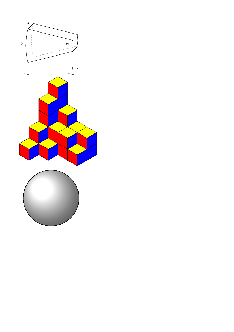
\begin{tikzpicture}
	% general shift to north east
	\coordinate (O) at (0.5,0.5);
	\draw[semithick] (0,0) -- (4,1);% bottom line in front
	\draw[dashed,color=gray] (O) -- ($(4,1)+(O)$);% bottom line in the back
	\draw[semithick] (0,3) -- (4,2);% top line in front
	\draw[semithick] ($(0,3)+(O)$) -- ($(4,2)+(O)$);% top line in the back
	\draw[semithick] (0,3) -- ($(0,3)+(O)$);% line to the back, top left
	\draw[semithick] (4,2) -- ($(4,2)+(O)$);% line to the back, top right
	\draw[semithick] (4,1) -- ($(4,1)+(O)$);% line to the back, bottom right
	\draw[dashed,color=gray] (0,0) -- (O);% line to the back, bottom left
	% the first angle is 180°+atan(0.25)
	% the second angle is 180°-atan(0.25)
	% the radius is sqrt(6^2+1.5^2)
	\draw[semithick] (0,0) arc (194.036:165.964:6.185);% left arc in front
	\draw[dashed,color=gray] (O) arc (194.036:165.964:6.185);% left arc in the back
	% the first angle is 180°+atan(0.25)
	% the second angle is 180°-atan(0.25)
	% the radius is 1/3*sqrt(6^2+1.5^2)
	\draw[semithick] (4,1) arc (194.036:165.964:2.062);% right arc in front
	\draw[semithick] ($(4,1)+(O)$) arc (194.036:165.964:2.062);% right arc in the back
	\draw (-0.5,1.7) node {$b_1$};
	\draw (3.6,1.7) node {$b_2$};
	\draw (0,3.5) node {$s$};
	\draw[|-,semithick] (0,-0.5) -- (4,-0.5);
	\draw[|->,semithick] (4,-0.5) -- (4.5,-0.5);
	\draw (0,-1) node {$x=0$};
	\draw (4,-1) node {$x=l$};
\end{tikzpicture}

%%%%%%%%%%%%%%%%%%%%%%%%%%%%%%%%%%%%%%%%%%%%%%%%%%%%%%%%%%%%%%%%%%%%%%%%%%%%%%%%%%%%%%%%%%%%%%%%%%%
% Three counters
\newcounter{x}
\newcounter{y}
\newcounter{z}

% The angles of x,y,z-axes
\newcommand\xaxis{210}
\newcommand\yaxis{-30}
\newcommand\zaxis{90}

% The top side of a cube
\newcommand\topside[3]{
  \fill[fill=yellow, draw=black,shift={(\xaxis:#1)},shift={(\yaxis:#2)},
  shift={(\zaxis:#3)}] (0,0) -- (30:1) -- (0,1) --(150:1)--(0,0);
}

% The left side of a cube
\newcommand\leftside[3]{
  \fill[fill=red, draw=black,shift={(\xaxis:#1)},shift={(\yaxis:#2)},
  shift={(\zaxis:#3)}] (0,0) -- (0,-1) -- (210:1) --(150:1)--(0,0);
}

% The right side of a cube
\newcommand\rightside[3]{
  \fill[fill=blue, draw=black,shift={(\xaxis:#1)},shift={(\yaxis:#2)},
  shift={(\zaxis:#3)}] (0,0) -- (30:1) -- (-30:1) --(0,-1)--(0,0);
}

% The cube
\newcommand\cube[3]{
  \topside{#1}{#2}{#3} \leftside{#1}{#2}{#3} \rightside{#1}{#2}{#3}
}

% Definition of \planepartition
% To draw the following plane partition, just write \planepartition{ {a, b, c}, {d,e} }.
%  a b c
%  d e
\newcommand\planepartition[1]{
 \setcounter{x}{-1}
  \foreach \a in {#1} {
    \addtocounter{x}{1}
    \setcounter{y}{-1}
    \foreach \b in \a {
      \addtocounter{y}{1}
      \setcounter{z}{-1}
      \foreach \c in {1,...,\b} {
        \addtocounter{z}{1}
        \cube{\value{x}}{\value{y}}{\value{z}}
      }
    }
  }
}


\begin{tikzpicture}
\planepartition{{5,3,2,2},{4,2,2,1},{2,1},{1}}
\end{tikzpicture}


%%%%%%%%%%%%%%%%%%%%%%%%%%%%%

\newcommand\pgfmathsinandcos[3]{%
  \pgfmathsetmacro#1{sin(#3)}%
  \pgfmathsetmacro#2{cos(#3)}%
}
\newcommand\LongitudePlane[3][current plane]{%
  \pgfmathsinandcos\sinEl\cosEl{#2} % elevation
  \pgfmathsinandcos\sint\cost{#3} % azimuth
  \tikzset{#1/.estyle={cm={\cost,\sint*\sinEl,0,\cosEl,(0,0)}}}
}
\newcommand\LatitudePlane[3][current plane]{%
  \pgfmathsinandcos\sinEl\cosEl{#2} % elevation
  \pgfmathsinandcos\sint\cost{#3} % latitude
  \pgfmathsetmacro\yshift{\cosEl*\sint}
  \tikzset{#1/.estyle={cm={\cost,0,0,\cost*\sinEl,(0,\yshift)}}} %
}
\newcommand\DrawLongitudeCircle[2][1]{
  \LongitudePlane{\angEl}{#2}
  \tikzset{current plane/.prefix style={scale=#1}}
   % angle of "visibility"
  \pgfmathsetmacro\angVis{atan(sin(#2)*cos(\angEl)/sin(\angEl))} %
  \draw[current plane] (\angVis:1) arc (\angVis:\angVis+180:1);
  \draw[current plane,dashed] (\angVis-180:1) arc (\angVis-180:\angVis:1);
}
\newcommand\DrawLatitudeCircle[2][1]{
  \LatitudePlane{\angEl}{#2}
  \tikzset{current plane/.prefix style={scale=#1}}
  \pgfmathsetmacro\sinVis{sin(#2)/cos(#2)*sin(\angEl)/cos(\angEl)}
  % angle of "visibility"
  \pgfmathsetmacro\angVis{asin(min(1,max(\sinVis,-1)))}
  \draw[current plane] (\angVis:1) arc (\angVis:-\angVis-180:1);
  \draw[current plane,dashed] (180-\angVis:1) arc (180-\angVis:\angVis:1);
}

%% document-wide tikz options and styles

\tikzset{%
  >=latex, % option for nice arrows
  inner sep=0pt,%
  outer sep=2pt,%
  mark coordinate/.style={inner sep=0pt,outer sep=0pt,minimum size=3pt,
    fill=black,circle}%
}


\begin{tikzpicture} % "THE GLOBE" showcase

\def\R{2.5} % sphere radius
\def\angEl{35} % elevation angle
\filldraw[ball color=white] (0,0) circle (\R);
\foreach \t in {-80,-60,...,80} { \DrawLatitudeCircle[\R]{\t} }
\foreach \t in {-5,-35,...,-175} { \DrawLongitudeCircle[\R]{\t} }

\end{tikzpicture}

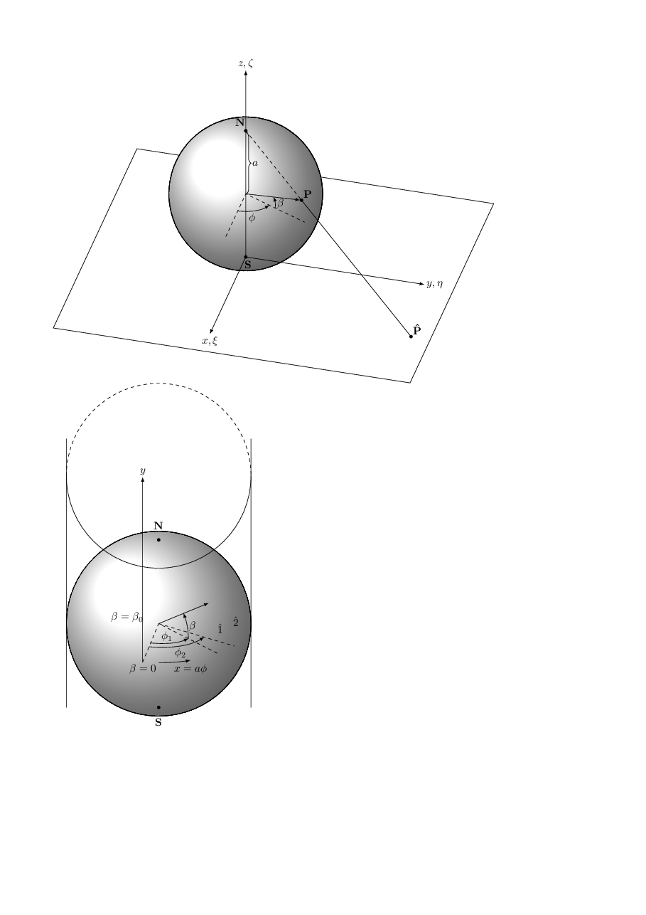
\begin{tikzpicture} % CENT

%% some definitions

\def\R{2.5} % sphere radius
\def\angEl{35} % elevation angle
\def\angAz{-105} % azimuth angle
\def\angPhi{-40} % longitude of point P
\def\angBeta{19} % latitude of point P

%% working planes

\pgfmathsetmacro\H{\R*cos(\angEl)} % distance to north pole
\tikzset{xyplane/.estyle={cm={cos(\angAz),sin(\angAz)*sin(\angEl),-sin(\angAz),
                              cos(\angAz)*sin(\angEl),(0,-\H)}}}
\LongitudePlane[xzplane]{\angEl}{\angAz}
\LongitudePlane[pzplane]{\angEl}{\angPhi}
\LatitudePlane[equator]{\angEl}{0}

%% draw xyplane and sphere

\draw[xyplane] (-2*\R,-2*\R) rectangle (2.2*\R,2.8*\R);
\fill[ball color=white] (0,0) circle (\R); % 3D lighting effect
\draw (0,0) circle (\R);

%% characteristic points

\coordinate (O) at (0,0);
\coordinate[mark coordinate] (N) at (0,\H);
\coordinate[mark coordinate] (S) at (0,-\H);
\path[pzplane] (\angBeta:\R) coordinate[mark coordinate] (P);
\path[pzplane] (\R,0) coordinate (PE);
\path[xzplane] (\R,0) coordinate (XE);
\path (PE) ++(0,-\H) coordinate (Paux); % to aid Phat calculation
\coordinate[mark coordinate] (Phat) at (intersection cs: first line={(N)--(P)},
                                        second line={(S)--(Paux)});

%% draw meridians and latitude circles

\DrawLatitudeCircle[\R]{0} % equator
%\DrawLatitudeCircle[\R]{\angBeta}
\DrawLongitudeCircle[\R]{\angAz} % xzplane
\DrawLongitudeCircle[\R]{\angAz+90} % yzplane
\DrawLongitudeCircle[\R]{\angPhi} % pzplane

%% draw xyz coordinate system

\draw[xyplane,<->] (1.8*\R,0) node[below] {$x,\xi$} -- (0,0) -- (0,2.4*\R)
    node[right] {$y,\eta$};
\draw[->] (0,-\H) -- (0,1.6*\R) node[above] {$z,\zeta$};

%% draw lines and put labels

\draw[dashed] (P) -- (N) +(0.3ex,0.6ex) node[above left] {$\mathbf{N}$};
\draw (P) -- (Phat) node[above right] {$\mathbf{\hat{P}}$};
\path (S) +(0.4ex,-0.4ex) node[below] {$\mathbf{S}$};
\draw[->] (O) -- (P) node[above right] {$\mathbf{P}$};
\draw[dashed] (XE) -- (O) -- (PE);
\draw[pzplane,->,thin] (0:0.5*\R) to[bend right=15]
    node[pos=0.4,right] {$\beta$} (\angBeta:0.5*\R);
\draw[equator,->,thin] (\angAz:0.4*\R) to[bend right=30]
    node[pos=0.4,below] {$\phi$} (\angPhi:0.4*\R);
\draw[thin,decorate,decoration={brace,raise=0.5pt,amplitude=1ex}] (N) -- (O)
    node[midway,right=1ex] {$a$};

\end{tikzpicture}

\begin{tikzpicture} % MERC

%% some definitions

\def\R{3} % sphere radius
\def\angEl{25} % elevation angle
\def\angAz{-100} % azimuth angle
\def\angPhiOne{-50} % longitude of point P
\def\angPhiTwo{-35} % longitude of point Q
\def\angBeta{33} % latitude of point P and Q

%% working planes

\pgfmathsetmacro\H{\R*cos(\angEl)} % distance to north pole
\LongitudePlane[xzplane]{\angEl}{\angAz}
\LongitudePlane[pzplane]{\angEl}{\angPhiOne}
\LongitudePlane[qzplane]{\angEl}{\angPhiTwo}
\LatitudePlane[equator]{\angEl}{0}

%% draw background sphere

\fill[ball color=white] (0,0) circle (\R); % 3D lighting effect
%\fill[white] (0,0) circle (\R); % just a white circle
\draw (0,0) circle (\R);

%% characteristic points

\coordinate (O) at (0,0);
\coordinate[mark coordinate] (N) at (0,\H);
\coordinate[mark coordinate] (S) at (0,-\H);
\path[xzplane] (\R,0) coordinate (XE);
\path[pzplane] (\angBeta:\R) coordinate (P);
\path[pzplane] (\R,0) coordinate (PE);
\path[qzplane] (\angBeta:\R) coordinate (Q);
\path[qzplane] (\R,0) coordinate (QE);

%% meridians and latitude circles

% \DrawLongitudeCircle[\R]{\angAz} % xzplane
% \DrawLongitudeCircle[\R]{\angAz+90} % yzplane
\DrawLongitudeCircle[\R]{\angPhiOne} % pzplane
\DrawLongitudeCircle[\R]{\angPhiTwo} % qzplane
\DrawLatitudeCircle[\R]{\angBeta}
\DrawLatitudeCircle[\R]{0} % equator

% shifted equator in node with nested call to tikz
% (I didn't know it's possible)
\node at (0,1.6*\R) { \tikz{\DrawLatitudeCircle[\R]{0}} };

%% draw lines and put labels

\draw (-\R,-\H) -- (-\R,2*\R) (\R,-\H) -- (\R,2*\R);
\draw[->] (XE) -- +(0,2*\R) node[above] {$y$};
\node[above=8pt] at (N) {$\mathbf{N}$};
\node[below=8pt] at (S) {$\mathbf{S}$};
\draw[->] (O) -- (P);
\draw[dashed] (XE) -- (O) -- (PE);
\draw[dashed] (O) -- (QE);
\draw[pzplane,->,thin] (0:0.5*\R) to[bend right=15]
    node[midway,right] {$\beta$} (\angBeta:0.5*\R);
\path[pzplane] (0.5*\angBeta:\R) node[right] {$\hat{1}$};
\path[qzplane] (0.5*\angBeta:\R) node[right] {$\hat{2}$};
\draw[equator,->,thin] (\angAz:0.5*\R) to[bend right=30]
    node[pos=0.4,above] {$\phi_1$} (\angPhiOne:0.5*\R);
\draw[equator,->,thin] (\angAz:0.6*\R) to[bend right=35]
    node[midway,below] {$\phi_2$} (\angPhiTwo:0.6*\R);
\draw[equator,->] (-90:\R) arc (-90:-70:\R) node[below=0.3ex] {$x = a\phi$};
\path[xzplane] (0:\R) node[below] {$\beta=0$};
\path[xzplane] (\angBeta:\R) node[below left] {$\beta=\beta_0$};

\end{tikzpicture}


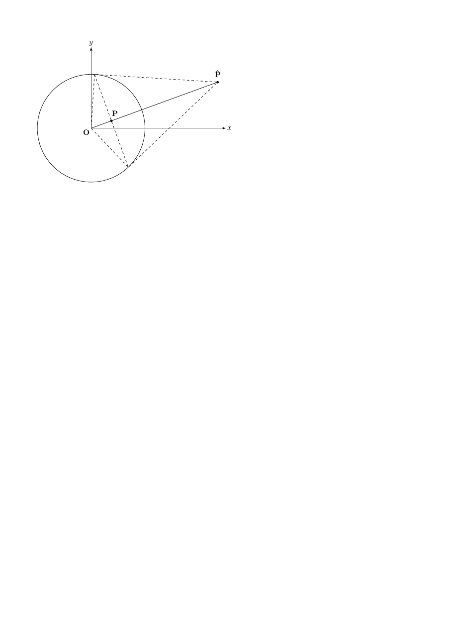
\begin{tikzpicture} % KART

\def\R{2.5}

\node[draw,minimum size=2cm*\R,inner sep=0,outer sep=0,circle] (C) at (0,0) {};
\coordinate (O) at (0,0);
\coordinate[mark coordinate] (Phat) at (20:2.5*\R);
\coordinate (T1) at (tangent cs: node=C, point={(Phat)}, solution=1);
\coordinate (T2) at (tangent cs: node=C, point={(Phat)}, solution=2);
\coordinate[mark coordinate] (P) at ($(T1)!0.5!(T2)$);

\draw[dashed] (T1) -- (O) -- (T2) -- (Phat) -- (T1) -- (T2);
\draw[<->] (0,1.5*\R) node[above] {$y$} |- (2.5*\R,0) node[right] {$x$};
\draw (O) node[below left] {$\mathbf{O}$} -- (P)
    +(1ex,0) node[above=1ex] {$\mathbf{P}$};
\draw (P) -- (Phat) node[above=1ex] {$\mathbf{\hat{P}}$};
\end{tikzpicture}

\end{document}